You Don’t Need Fine-Tuning an Embedding Model – Building a Summer Embedding Lens for Fashion E-commerce Search

Imagine if your product-search engine could sense the change of seasons the same way a shopper does, or know about memorable moments, instantly swapping wool coats for sundresses the moment summer hits, or spotlighting perfect gift ideas in the run-up to Mother’s Day. That’s the promise of Embedding Lens, a plug-and-play “spectacles” layer that slips over any static embedding model and teaches it new tricks without costly reprocessing.

What Static Re-indexing Can’t Fix 🎯

The typical search pipeline already reindexes every new or edited SKU overnight, so the catalog itself is always up to date. What isn’t fresh are the context signals, those short-lived moments when customers want a different flavour of “relevance” without any change in product data.

Context moment	User query	User wish	Why the encoder can’t keep up
Early summer	bag	Raffia, canvas, brights	Embeddings learned on season-agnostic data.
Christmas gifts	mini bag	Sparkly, party-ready	Model still ranks everyday leather first.
Mother’s Day	scarf	Floral, gift-boxed	Needs a temporary giftable bias.

Re-training or re-ranking for every event is overkill, slow, GPU-hungry, and risk-heavy in prod.

We need a surgical dial that we can turn on/off per query, per segment, or per campaign without touching product information (description or embeddings).

Our Angle: the Embedding Lens 👓

What’s an Embedding Lens?

A tiny linear map T we multiply with the query embedding right before the nearest-neighbor lookup:

\[\tilde{q} = \text{norm}((I + UV^{\top}) q); \quad U, V \in \mathbb{R}^{d \times r}, \, r \ll d.\]

• In plain English: “Nudge the query toward specific criteria in the embedding space.”
• Zero changes to product information, zero re-indexing.

Label once, Use Forever: We only need to label a product set to train the lens. Once the lens understands the target concept, it can be applied to new products without requiring modifications to the catalog.

Why start with a Summer lens?

• Seasonality is an easy win - When the weather changes, so does what “relevant” looks like; stakeholders feel the impact immediately.
• Seasonality is complex enough - To determine a product is suitable for summer requires taking into account many aspects of the product not just a linear relation to a particular characteristic.
• Instant visual sanity-check - “raffia tote > leather tote” is obvious at first glance, letting us iterate quickly before tackling subtler segments.
• Perfect sandbox for the bigger goal - If a single lens can nudge search toward beach-ready styles, the same trick can later target gifting, vegan, or city-specific intent without adding any additional information to products.

How We Built It 🔧

Mind-set: Start small, validate early and then scale

Idea spark

The initial thought was modest: “What if we steer only the search vector instead of updating every product embedding?” A quick literature sweep (adapters, prompt-tuning, linear query shifts) confirmed the maths was already out there, waiting to be applied.

The shortest way to validate (The “Red” Lens)

To test the waters, we took a frozen snapshot of the full catalogue and trained a lens on roughly 300 triplets (red versus non-red), small enough to run on a laptop’s CPU. A handful of sample queries (“bag”, “sneakers”, “dress”) instantly floated scarlet items to the top 3: plenty of signal, zero re-indexing.

Testing the “summer” waters

When the business team identified seasonality as a significant challenge, we revised the pipeline. We replaced the previous red-not-red dataset with a summer label generated using a large language model (LLM) and rebuilt the triplet file based on the current catalog. All other elements, including the data format and training code, stayed the same.

Understanding Summer Vibes (Lab-scale validation)

After validating our hypothesis with a small model, we aimed to scale up and determine if it could be applied to a production-grade system. To achieve this, we created an equivalent lab environment suited for testing and validation.

Utilizing the complete product set and real query logs, we transitioned to using a single rented GPU (from Runpod) and trained an image-and-text-based summer lens model. We then measured performance using Precision@k, Summer-Precision@k, and latency metrics (in W+B).

Over several iterative cycles, spread across spare evenings and quiet mornings, we tuned hyperparameters until the semantic gains were consistent and the added latency stayed within acceptable limits for production.

The Recipe: Crafting a Consistent Training Routine for a Beach-Ready Model

Data preparation

Before an AI model can effectively adapt embeddings for semantic search, it needs a well-structured and informative training dataset. In this phase, we assemble aligned pairs of user queries and products, along with their respective vector embeddings and a supervision signal that guides the learning process.

Our target schema captures the key components for this adaptation process:

{
  "query": "search text query",
  "query_embedding": "embedding representation of the query",
  "product_id": "unique identifier of the product",
  "product_embedding": "embedding representation of the product",
  "len_score": "adjustment parameter indicating the desired similarity level"
}

Each row represents a training example linking a natural language query to a candidate product. The len_score field encodes how closely the embeddings should align in semantic space, enabling the model to learn a fine-tuned transformation that reflects domain-specific relevance.

Let’s break down the different components and illustrate how the data is collected and transformed to fit the target schema.

1. Queries

The query field is sourced from real user behavior in production analytics. We focus on the most commonly used and semantically rich queries issued by users in the existing system. These high-frequency queries help the model learn patterns that generalize well to real-world search behavior.

2. Products

Each product_id maps to a product entry retrieved from the production database. We ensure the product metadata, including titles, descriptions, and image references, is up to date and consistent with what users see in the current search experience.

3. Embeddings

The query_embedding and product_embedding fields are generated using the same embedding strategy deployed in production to maintain consistency within the semantic space.

• Product Embedding = CLIP LAION (on product images) + text-embedding-3-large (on product description)
• Query Embedding = CLIP LAION (on query text) + text-embedding-3-large (on query text)

By concatenating multimodal embeddings from both vision (CLIP) and text (OpenAI), we create a joint semantic space that captures visual style and textual meaning, essential for fashion and lifestyle domains where style matters as much as substance.

4. Len Score

The len_score is a synthetic supervision signal indicating how semantically close a product should be to the query in the adapted embedding space. It is generated using a custom large language model (LLM) classifier trained to recognize alignment with seasonal style cues (e.g., “summer vibes”, “beachwear”, “light fabrics”).

To scale this process efficiently, we use OpenAI Batches, allowing us to label thousands of products at once. Then, we rank each product based on its summer score and semantic similarity to each query. This enables the creation of a rich, style-aware training dataset without manual labeling bottlenecks.

Protecting Semantic Integrity

While adapting embeddings for nuanced relevance, it’s critical not to break the core semantic integrity of the search space. For example, a high-scoring summer “bikini swimsuit” should never appear at the top of results for a query like “bags”, no matter how stylistically aligned.

To safeguard against this, we introduced a similarity gate: A function that, if a product is fundamentally unsuitable for a given query category, the len_score is forcibly set to 0, turning that pair into a contrastive negative during training. This ensures that adaptation enhances style relevance without sacrificing semantic precision.

Final dataset

To support training and evaluation at scale, we compiled a robust and diverse dataset using a combination of production analytics, embedding-based filtering, and random sampling.

Queries:

• 1,300 high-frequency search queries, extracted from real user behavior.

Products per Query:

• 500 top-ranked products based on baseline cosine similarity using the current (unadapted) embedding space.
• 500 randomly selected products from the remainder of the 16,000-product catalog to introduce semantic diversity and harder negatives.

Total: ~1.3 million query-product pairs

Data Split:

• 60% Training Set – used to fit the transformation model.
• 40% Evaluation Set – used to measure generalization and assess model performance against held-out queries and products.

By combining both relevant and irrelevant candidates per query, this helps the model learn fine-grained distinctions in style relevance.

This structured and automated data preparation pipeline ensures that our adaptation model is trained on relevant, high-quality signals that are grounded in production semantics and enhanced with domain-specific relevance cues. In the next section, we will explore how this dataset is utilized to train a lightweight projection module, which subtly adjusts embeddings to better align with user expectations in seasonal and style-driven contexts.

Training pipeline

With our data prepped and aligned, the next step is training the model to learn a fine-grained transformation that shifts query embeddings just enough to reflect user intent and seasonal trends—without breaking the underlying semantic alignment.

Model Architecture

At the heart of our system is a lightweight neural network that learns to apply a small but meaningful delta to the original query embedding:

class EmbeddingTransformer(nn.Module):
    def __init__(self, dim, hidden_dim):
        super().__init__()
        self.transform = nn.Sequential(
            nn.Linear(dim, hidden_dim),
            nn.ReLU(),
            nn.Dropout(0.1),
            nn.Linear(hidden_dim, dim)
        )

    def forward(self, x):
        delta = self.transform(x)
        return delta

This architecture takes an input query embedding of dimension 4352 (concatenated CLIP and text embeddings) and learns a residual-style projection. The output delta is added back to the original embedding and normalized, forming the adapted query vector used for training.

Loss Function: Cosine Similarity Regression

To align the adapted query vector with the target product embedding, we use a cosine similarity regression loss, scaled from [-1, 1] to [0, 1] and compared to the len_score target via Mean Square Error (MSE):

def _cosine_similarity_regression_loss(self, q, p, target):
    p_normalized = F.normalize(p, dim=-1)
    cos_sim = (F.cosine_similarity(q, p_normalized, dim=-1) + 1) / 2
    return F.mse_loss(cos_sim, target)

This lets the model learn how similar a product should be to a given query, not just a binary match, but a nuanced similarity score that reflects stylistic intent.

Training Loop and Monitoring

We train the model using PyTorch and the Adam optimizer, with all metrics logged via Weights & Biases (W&B) for real-time monitoring.

To streamline training, manage hardware resources (in Runpod) more efficiently, and gain more granular control over the training process, we updated the loop to use the Hugging Face Accelerate framework.

This allows us to:

• Efficiently scale across devices (CPU/GPU)
• Better manage memory usage for large embeddings
• Easily swap data strategies during experimentation

Here’s how it works:

• Load query-product pairs from the training dataset (jsonl format).
• Each epoch processes query-product pairs in batches:
  • Generate the delta and add it to the original query embedding.
  • Normalize the new query vector.
  • Compute cosine similarity with the product embedding.
  • Back propagate using MSE loss between similarity and len_score.
• Log training loss per step and average loss per epoch to W&B.
• Save model checkpoints after each epoch with timestamped filenames.
• Upload final metrics including loss, elapsed time, and model path to W&B at the end of training.

This setup enables:

• Fast experimentation with consistent model saving and tracking.
• Simple restart or resume of training from checkpoints.
• Easy inspection of model behavior and convergence across epochs.

Lens Usage

Once the Summer Lens model is trained, it can be applied in real time to adapt incoming query embeddings, subtly shifting their position in the semantic space to favor seasonal or stylistic intent without losing category relevance.

The process is lightweight and fast, making it suitable for production environments:

query_tensor = torch.tensor(query_embedding, dtype=torch.float32).reshape(1, -1)

delta = self.model(query_tensor)
adapted_query_embedding = F.normalize(query_tensor + delta, dim=-1)

The adapted embedding is then utilized in the vector search pipeline just like the original one, enhancing the relevance of results for queries influenced by seasonality and style.

This “lens” functions as a lightweight, plug-and-play, differentiable filter over the original query, adjusting its representation to better align with what users are truly seeking, particularly in areas where intent may change over time, trends, or context.

Need a different trade‑off?

When you want to maintain more of the original query’s meaning while still incorporating seasonal or stylistic adjustments, consider blending the raw and adapted embeddings.

You can do this by adjusting the blend factor α (where q_final = (1‑α)·q_raw + α·q_lens) to achieve the desired level of seasonal bias without needing to retrain or re-index:

alpha = 0.7 # Blending factor

weighted_query = F.normalize((1-alpha) * query_emb + alpha * adapted_query_emb, dim=-1)

This gives you finer control over how much influence the lens has, enabling gradual adaptation instead of full transformation, especially useful for sensitive or high-precision search scenarios.

Evaluation & Validation pipeline

Our eyes and intuition indicated that our approach was effective, but we needed formal validation to confirm its efficacy for implementation in a production environment. The best part is that if this technique is validated, we can incorporate it into our toolkit for future projects, which will save time and money by allowing us to bypass unnecessary fine-tuning loops while still achieving excellent results.

We promised ourselves two things before giving this as validated:

1. Keep the score-card tiny. One number for general relevance, one for summer vibes.
2. Automate the whole pass. Hit Enter, come back to a W&B dashboard.

What we measure

Metric	Why we care	Threshold we locked
Precision @ k	“Of the first k results, how many are simply relevant?”	Count how many of the top-k items cross the same relevance score the baseline already meets (we freeze that cut-off at 0.67).
Summer-Precision @ k	“Of those k, how many really scream summer?”	Ask an LLM to rate each product 0-1 on “summer vibe”. Anything ≥ 0.70 counts as a beach-hit and bumps the score

Both metrics are averaged over the evaluation split of hold-out production queries that have not been included in the training loop.

How the evaluation works

from seasonal_lens.common.metrics import (
    load_search_results,        # jsonl → {query: [ids]}
    load_scores_from_jsonl,     # jsonl → {query: {id: score}}
    precision_at_k
)
import numpy as np
from pathlib import Path

# --- 1. Load artefacts ----------------------------------------------------
variant   = load_search_results(Path("results/lens.jsonl"))
relevance = load_scores_from_jsonl(Path("labels/relevance.jsonl")) # cosine
summer    = load_scores_from_jsonl(Path("labels/summer.jsonl"))    # 0-1 summer-score

# --- 2. Compute metrics ---------------------------------------------------
def mean_prec(results, labels, thr, k=5):
    return np.mean([
        precision_at_k(
            [labels[q].get(pid, 0.0) for pid in ranks],
            k=k,
            threshold=thr
        )
        for q, ranks in results.items()
    ])

prec5        = mean_prec(variant, relevance, thr=0.67, k=5)
summer_prec5 = mean_prec(variant, summer,    thr=0.70, k=5)

print(f"Precision@5        : {prec5:.3f}")
print(f"Summer-Precision@5 : {summer_prec5:.3f}")

def precision_at_k(scores, k, thr):
    hits = sum(s >= thr for s in scores[:k])
    return hits / k

1. Generates a baseline ranking straight from relevance labels
2. Loads the lens runs
3. Computes Precision @ k and Summer-P @ k for both the baseline and the lens
4. Logs results to W&B

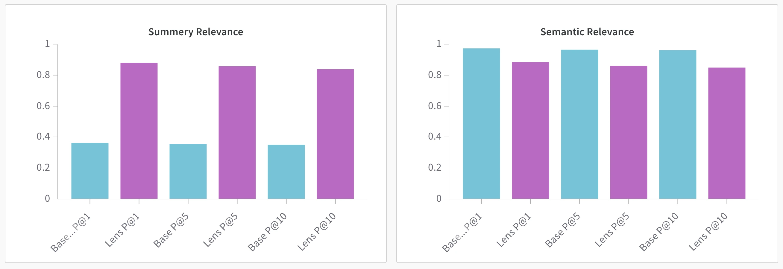
The numbers: Decoding the Results 📊

After training and evaluation, the results confirmed the value of embedding adaptation through the Summer Lens. The best-performing setup used a 50/50 blend of the original and adapted query vectors, successfully capturing the seasonal relevance boost without sacrificing the baseline precision.

Even better, performance remained production-ready: added latency averaged just 1.04 ms per query, making the lens suitable for real-time search pipelines with no noticeable overhead.

Best-performing setup results

1. Summer catalog boost: +138,4%
2. Overall relevance impact: -11,71%

Metrics comparison between the baseline model and the applied lens model

Results snapshot

Metric	Baseline	Lens 100%	Lens 50% blend
Precision @ 10	0.96	0.58	0.86
Summer-P @ 10	0.35	0.95	0.86
Extra Latency (ms)	-	1.04	1.04

What We Learned (Tips) 🎓

1. Cheap synthetic data is gold. OpenAI batch prompts gave us realistic, summer scores for all the catalog items (11k) in less than a day.
2. Screenshots trump spreadsheets. Putting results side‑by‑side makes the shift instantly clear to business stakeholders, far better than dropping a table of numbers, so every evaluation run now auto‑exports that comparison image.
3. Trust, but eyeball. When we build the len_score (relevance + summer vibe), the weightings can accidentally tip the scale, everything looks “very summer” or “hardly summer” at all. A quick histogram of those combined scores shows how much variety we really have on the summer axis, so we can rebalance triplets before training and avoid teaching the lens a one‑note view of the catalogue
4. Blending is a secret weapon. That extra knob α lets us decide how much lens power to apply, α = 0.5 hit the sweet spot and saved days of hyper‑param tinkering and code churn.
5. Version everything. We store triplet files and LLM scores on Hugging Face Datasets; rolling back a bad run is just changing a dataset tag.

Conclusions 🎯

The Embedding Lens proves that contextual search can be made both agile and production‑ready. By adding a lightweight, toggleable layer to our existing embedding pipeline, we can deliver seasonally or thematically tailored results without re‑indexing, retraining the base model, or adding operational complexity, while preserving production‑grade performance and simple deployments at scale.

Key takeaways:

• On‑demand adaptation: Activate or retire themed search experiences in seconds, no catalog reprocessing required.
• Faster data prep: LLM‑generated synthetic data cuts human labeling effort, enabling rapid rollout of new lenses aligned to business needs.
• Rapid, low‑cost iteration: The lens architecture trains economically, supporting quick prototype-test-refine cycles.
• Production‑safe latency: ~1.04 ms added per query, effectively negligible for user experience.
• Risk‑mitigated rollout: Straightforward A/B testing lets us trial multiple themed searches across segments without infrastructure changes.
• Built for extensibility: Supports lens composition (e.g., “summer+party”), multi‑aspect context (weather, location), and behavior‑adaptive lenses, without retraining the foundational embedding model.

Overall, the embedding lens approach advances our search architecture toward a more responsive, context‑aware system that scales operationally and economically, making continuous innovation practical in production.